Demand Forecast of Retail Products Using ARIMA Method
In this comprehensive analysis, I embarked on a journey to enhance the inventory management and sales strategy of eOptika, a European international optical product retailer and webshop chain. By leveraging sophisticated statistical and machine learning methods, I aimed to accurately forecast product demand mostly in order to optimize investment in stock inventory. At the first phase of the project, I focused on product level (instead of product group, brand or manufacturer level). The forecast spanned from January 2018 to February 2024, providing invaluable insights for strategic planning and operational efficiency.
Table of contents
- 00. Project Overview
- 01. Data Acquisition & Preprocessing
- 02. Forecasting Models Implementation
- 03. Model Evaluation & Selection
Project Overview
Context
In the rapidly evolving retail environment, eOptika faced challenges in maintaining optimal stock levels across its stores nationwide. Excess inventory leads to increased holding costs, while stockouts risk losing sales and customer satisfaction. Addressing this challenge, our project focuses on forecasting the demand for the whole product line, which has shown variable sales patterns over recent years.
Actions
To develop a reliable demand forecasting model that predicts monthly sales for each product sold by the retailer. To provide actionable insights for inventory management and sales strategies, reducing holding costs and minimizing stockouts.
Methodology Overview
Utilizing Python’s sqlalchemy library, I performed data extraction from eOptika’s MySQL database, followed by data preprocessing to ensure quality and consistency. I then explored various forecasting models, namely AutoARIMA and ETS, and LSTM to capture the underlying sales trends and seasonality. The models were evaluated based on Root Mean Squared Error (RMSE), guiding us to the best-fit model for eOptika.
Data Acquisition & Preprocessing
The project commenced with establishing a secure connection to eOptika’s analytics database:
# Create database connection
from sqlalchemy import create_engine
engine = create_engine('mysql+pymysql://user:pwsd@10.1.11.1:5555/eoptika_analytics')
con = engine.connect()
After reaching out to the database, I extracted historical sales data on a product level. Since this has been a univariate analysis, all I needed were a temporal variable, “month”, and the measure that I wanted to forecast, “items_sold (units)”.
A sample of this data (the first 5 rows) can be seen below:
| product | month | items_sold (units) |
|---|---|---|
| 1 Day Acuvue Moist (30) | 2018-01 | 498 |
| 1 Day Acuvue Moist (30) | 2018-02 | 387 |
| 1 Day Acuvue Moist (30) | 2018-03 | 454 |
| 1 Day Acuvue Moist (30) | 2018-04 | 473 |
| 1 Day Acuvue Moist (30) | 2018-05 | 539 |
Ezt itt el kell magyarázni, hogy mi a szart csinál:
    # Rename columns and preprocess data
    sales_data = sales_data.rename(columns={'months': 'ds', 'sales': 'y'})
    sales_data['y'] = sales_data['y'].astype(float)
    sales_data['ds'] = pd.to_datetime(sales_data['ds']) + MonthEnd(1)
    sales_data = sales_data.assign(unique_id=0).set_index('unique_id')
Forecasting Models Implementation
My plan was to compare the performace of 3 models: (1) SARIMA model with using python’s AutoARIMA forecasting model, (2) Exponential Smoothing using ETS, and LSTM, which belong to the class of a deep learning methods. Since LSTM requires a different data preparation, I left it out from the first attempt to get forecasts. The SARIMA model was implemented by Python’s AutoARIMA that automatically identifies the best ARIMA model parameters, while Exponential Smoothing was leveraged by Python’s ETS (Error term, Trend component and Seasonal component) library.
This is how the code snippet looks like that handles data preparation, train-test-split and training the models:
# Assuming all_data is your DataFrame with 'CT2_pack', 'months', and 'sales' columns
unique_ct2_packs = all_data['CT2_pack'].unique()

for ct2_pack in unique_ct2_packs:
    # Filter data for the current CT2_pack
    sales_data = all_data[all_data['CT2_pack'] == ct2_pack].copy()

    # Rename columns and preprocess data
    sales_data = sales_data.rename(columns={'months': 'ds', 'sales': 'y'})
    sales_data['y'] = sales_data['y'].astype(float)
    sales_data['ds'] = pd.to_datetime(sales_data['ds']) + MonthEnd(1)
    sales_data = sales_data.assign(unique_id=0).set_index('unique_id')

    # Split data into training and testing (select only the 2nd and 3rd columns)
    Y_train_df = sales_data.iloc[:-6, 1:3]
    Y_test_df = sales_data.iloc[-6:, 1:3]

    season_length = 12
    horizon = len(Y_test_df)

    models = [
        AutoARIMA(season_length=season_length),
        ETS(season_length=season_length)
    ]

    model = StatsForecast(
        df=Y_train_df,
        models=models,
        freq='M'
    )

    Y_hat_df = model.forecast(horizon)

    # Accuracy Metrics and Plotting
    for model_name in ['AutoARIMA', 'ETS']:  # ETS is the Exponential Smoothing
        Y_true = Y_test_df['y'].values  # Actual values
        Y_pred = Y_hat_df[model_name].values  # Predicted values from your forecast

        # Calculate accuracy metrics
        mse = mean_squared_error(Y_true, Y_pred)
        rmse = np.sqrt(mse)

        # Print the accuracy metrics
        print(f'Accuracy Metrics for {ct2_pack} using {model_name}:')
        print(f'Root Mean Squared Error (RMSE): {rmse:.2f}')
        print(f'RMSE per Mean Actual Sales Values from Test Period: {rmse/Y_true.mean():.2f}')
Model Evaluation & Selection
Comparing SARIMA and Exponential Smoothing
First, I wanted to test two traditional models, SARIMA and Exponential Smoothing to select the one that best captured the sales trends and offered the highest accuracy for the forecasts.
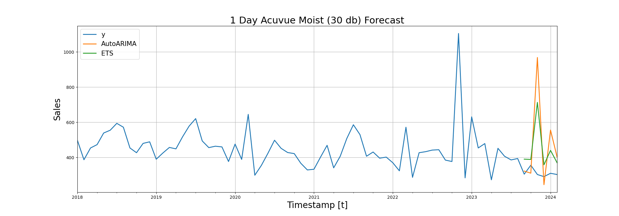
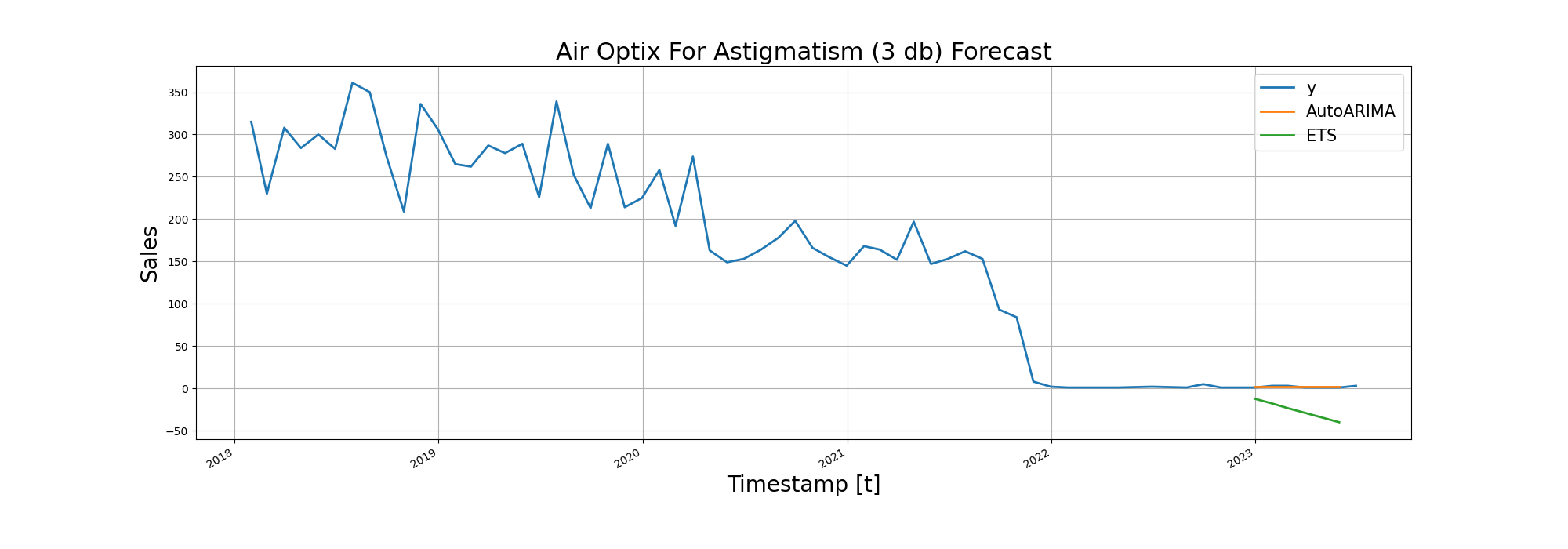
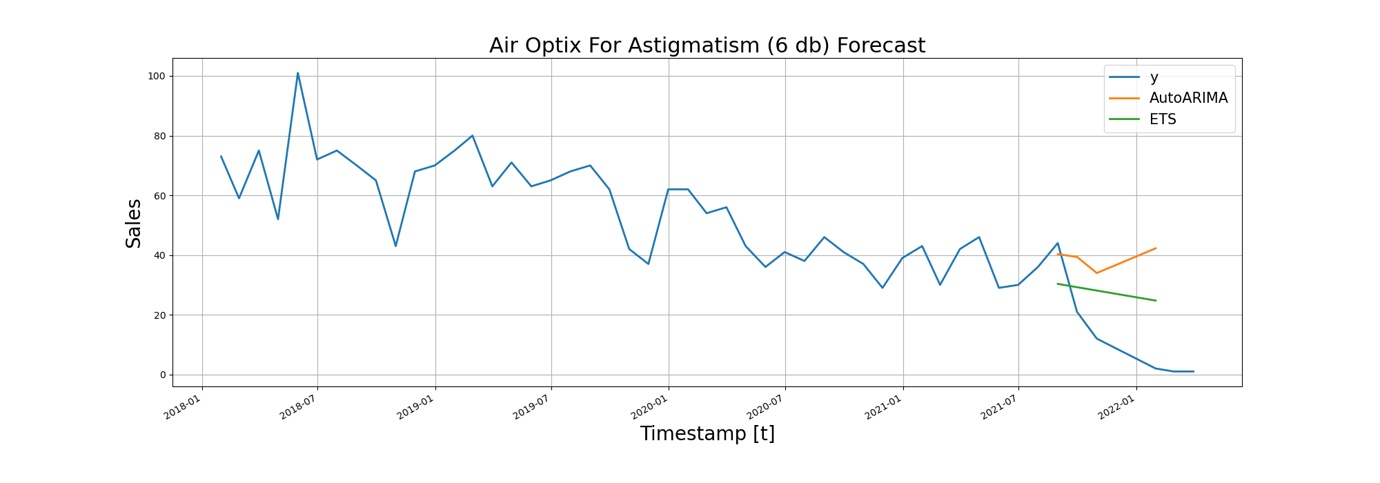
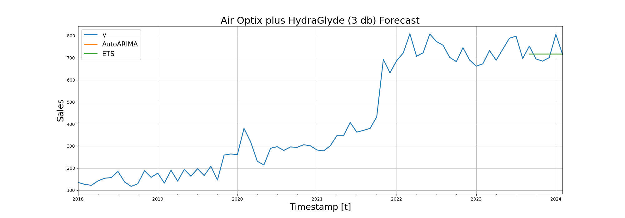
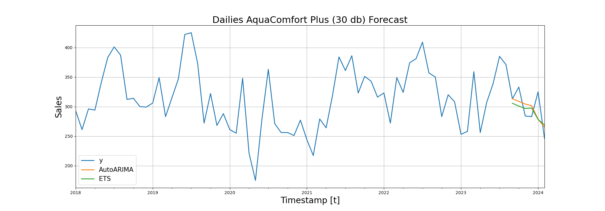
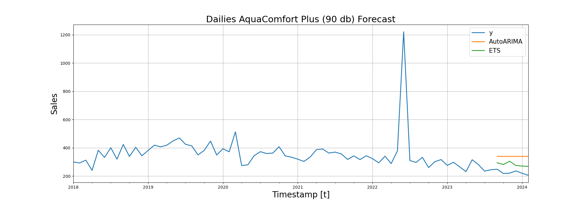
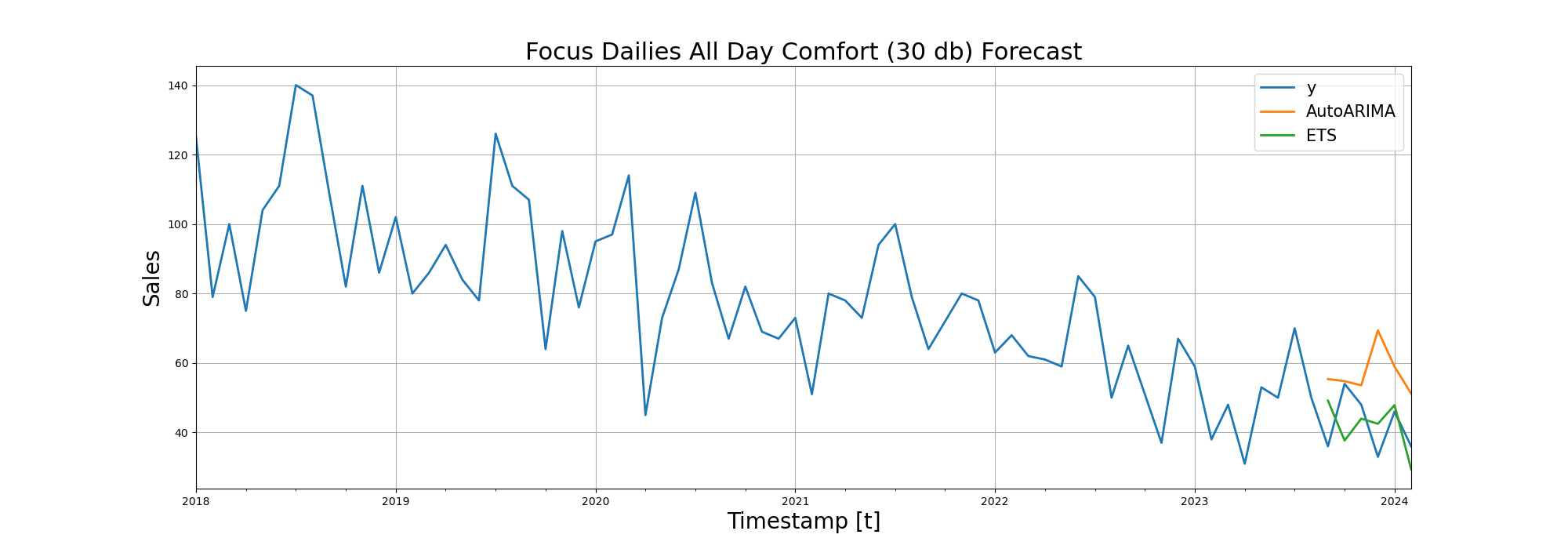
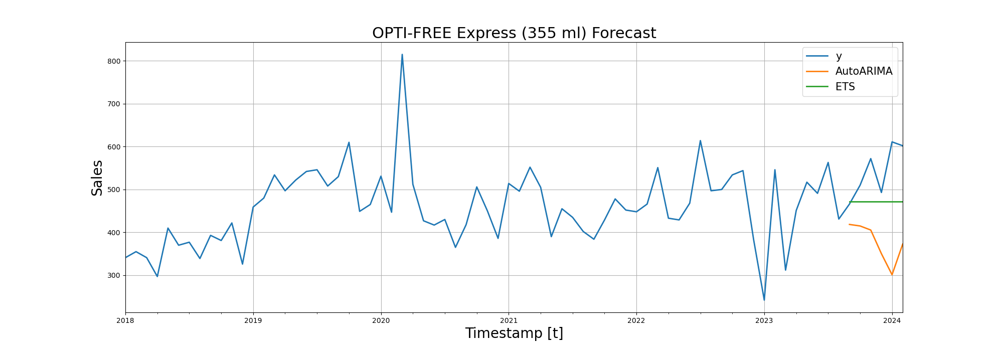
From the table below, we can see that SARIMA and Exponential Smoothing perform in a very similar manner. I would personally pick Exponential Smoothing since it won the duel at more products.
RMSE values for the product by models look like this:
| Product | SARIMA (RMSE) | Exponential Smoothing (RMSE) |
|---|---|---|
| 1 Day Acuvue Moist (30) | 293.72 | 183.69 |
| Air Optix For Astigmatism (3) | 1.05 | 29.76 |
| Air Optix For Astigmatism (6) | 27.46 | 19.66 |
| Air Optix plus HydraGlyde (3) | 42.58 | 42.6 |
| Air Optix plus HydraGlyde (6) | 40.6 | 67.59 |
| Air Optix plus HydraGlyde for Astigmatism (3) | 41.23 | 39.55 |
| Biofinity (3) | 641.56 | 573.33 |
| Biofinity (6) | 853.41 | 750.15 |
| Dailies AquaComfort Plus (30) | 25.37 | 26.36 |
| Dailies AquaComfort Plus (90) | 114.97 | 59.44 |
| Focus Dailies All Day Comfort (30) | 18.84 | 9.94 |
| OPTI-FREE Express (355 ml) | 186.21 | 90 |
| Systane Ultra (10 ml) | 109.16 | 109.07 |
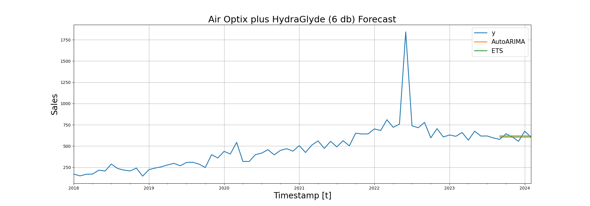
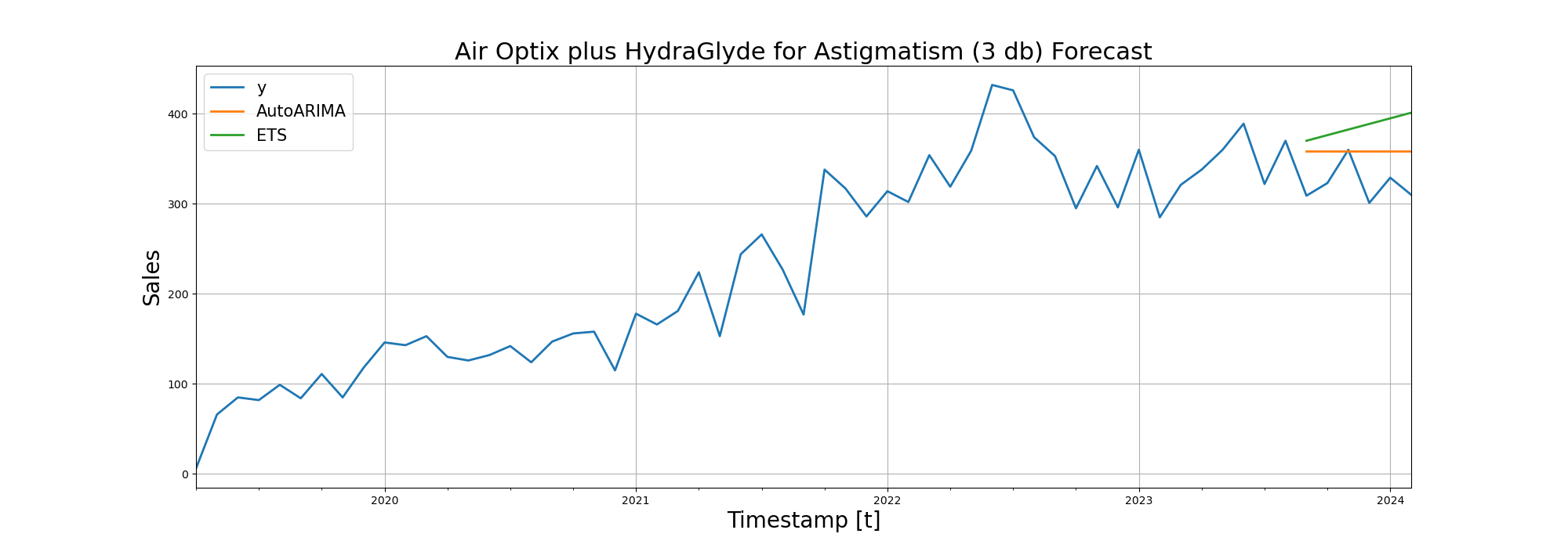
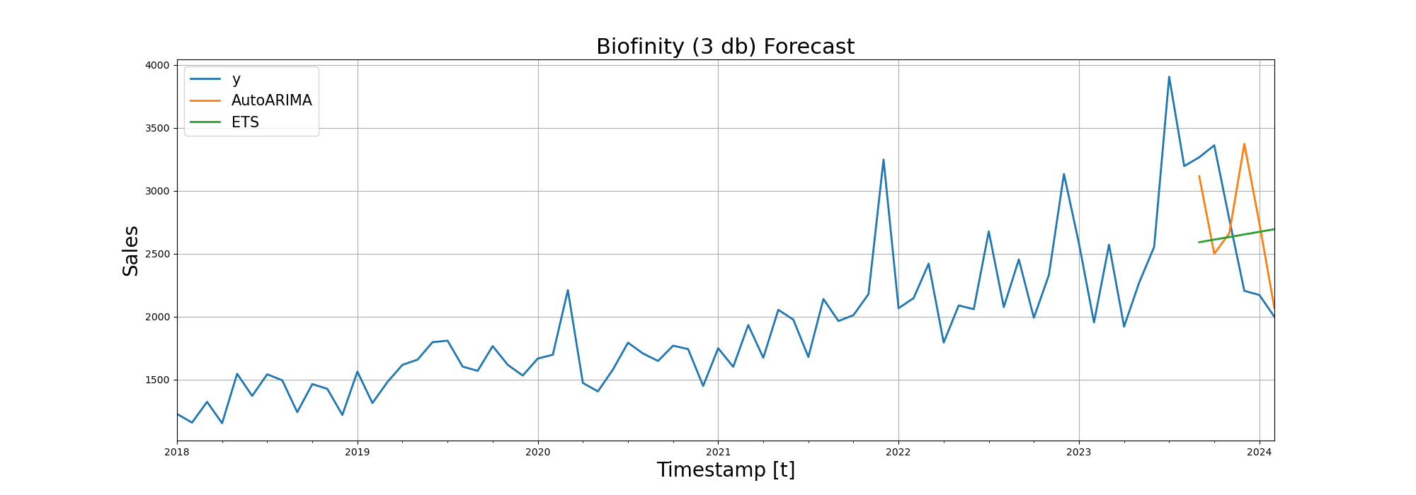
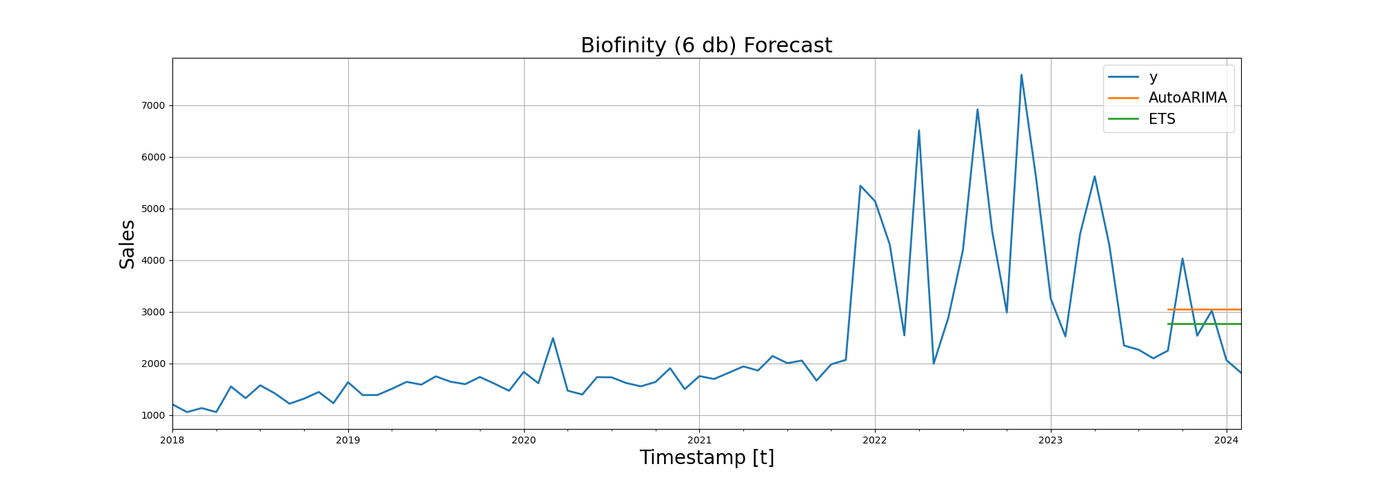
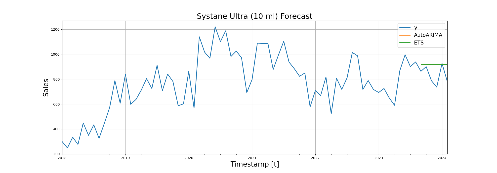
After RMSE (Root Mean Squared Error), we visualized the forecasting performance of the models on line diagrams:
Trying Deep Learning in Time Series Forecasting
After applying 2 traditonal techniques, I turned to deep learning to see if it can capture nuance drivers of the sales demand movements on top of trend and seasolality.
The following code snippet demonstrates a process for forecasting sales data using an LSTM neural network in TensorFlow. It begins by filtering and preprocessing sales data for unique product packs, normalizing the data, and then creating a dataset with a specified number of time steps to be used for training and testing the LSTM model. Finally, the model is built, compiled, and fitted with the training data, followed by predictions on the test set, with the performance evaluated using the root mean squared error (RMSE) metric for each product pack:
from tensorflow.keras.models import Sequential
from tensorflow.keras.layers import LSTM, Dense

# Function to prepare data for LSTM
def create_dataset(X, y, time_steps=1):
    Xs, ys = [], []
    for i in range(len(X) - time_steps):
        v = X.iloc[i:(i + time_steps)].values
        Xs.append(v)
        ys.append(y.iloc[i + time_steps])
    return np.array(Xs), np.array(ys)

unique_ct2_packs = all_data['CT2_pack'].unique()

for ct2_pack in unique_ct2_packs:
    # Filter and preprocess data
    sales_data = all_data[all_data['CT2_pack'] == ct2_pack]
    sales_data = sales_data.rename(columns={'months': 'ds', 'sales': 'y'})
    sales_data['ds'] = pd.to_datetime(sales_data['ds']) + MonthEnd(1)

    # Normalize the data
    scaler = MinMaxScaler(feature_range=(0, 1))
    sales_data_scaled = scaler.fit_transform(sales_data[['y']])

    # Preparing dataset for LSTM
    time_steps = 12
    X, y = create_dataset(pd.DataFrame(sales_data_scaled), pd.DataFrame(sales_data_scaled), time_steps)

    # Keeping the last 6 months for testing
    train_size = len(X) - 6
    X_train, X_test = X[:train_size], X[-6:]
    y_train, y_test = y[:train_size], y[-6:]

    # Build LSTM model
    model = Sequential([
        LSTM(50, activation='relu', input_shape=(time_steps, 1)),
        Dense(1)
    ])
    model.compile(optimizer='adam', loss='mean_squared_error')

    # Fit model
    model.fit(X_train, y_train, epochs=200, batch_size=32, verbose=0)

    # Predict
    y_pred = model.predict(X_test)
    y_test_inv = scaler.inverse_transform(y_test)
    y_pred_inv = scaler.inverse_transform(y_pred)

    # Calculate metrics
    mse = mean_squared_error(y_test_inv, y_pred_inv)
    rmse = np.sqrt(mse)

    # Print metrics
    print(f'RMSE for {ct2_pack} using LSTM: {rmse:.2f}')

    # Plotting the results
    plt.figure(figsize=(10, 6))
    plt.plot(range(len(y)), scaler.inverse_transform(y), label="True", alpha=0.75)
    plt.plot(range(len(y_train), len(y)), y_test_inv.flatten(), marker='.', label="Actual")
    plt.plot(range(len(y_train), len(y)), y_pred_inv.flatten(), 'r', label="Predicted")
    plt.ylabel('Sales')
    plt.xlabel('Time Step')
    plt.legend()
    plt.show()
RMSE values for the product by models including LSTM look like this:
| Product | SARIMA (RMSE) | Exponential Smoothing (RMSE) | LSTM (RMSE) |
|---|---|---|---|
| 1 Day Acuvue Moist (30) | 293.72 | 183.69 | 133.45 |
| Air Optix For Astigmatism (3) | 1.05 | 29.76 | 1.62 |
| Air Optix For Astigmatism (6) | 27.46 | 19.66 | 22.07 |
| Air Optix plus HydraGlyde (3) | 42.58 | 42.6 | 51.02 |
| Air Optix plus HydraGlyde (6) | 40.6 | 67.59 | 138.31 |
| Air Optix plus HydraGlyde for Astigmatism (3) | 41.23 | 39.55 | 32.12 |
| Biofinity (3) | 641.56 | 573.33 | 1538.74 |
| Biofinity (6) | 853.41 | 750.15 | 965.48 |
| Dailies AquaComfort Plus (30) | 25.37 | 26.36 | 37.65 |
| Dailies AquaComfort Plus (90) | 114.97 | 59.44 | 121.58 |
| Focus Dailies All Day Comfort (30) | 18.84 | 9.94 | 8.09 |
| OPTI-FREE Express (355 ml) | 186.21 | 90 | 79.27 |
| Systane Ultra (10 ml) | 109.16 | 109.07 | 82.11 |
We can conclude that LSTM does not excel over the other 2 traditional models.